Hello world! Last summer I wrote a short paper entitled "Entropy as a Topological Operad Derivation," which describes a small but interesting connection between information theory, abstract algebra, and topology. I blogged about it here in June 2021, and the paper was later published in an open-access journal called Entropy in September 2021. In short, it describes a correspondence between Shannon entropy and functions on topological simplices that obey a version of the Leibniz rule from calculus, which I call "derivations of the operad of topological simplices," hence the title.

By what do those words mean? And why is such a theorem interesting?

‍To help make the ideas more accessible, I've recently written a new article aimed at a wide audience to explain it all from the ground up. I'm very excited to share it with you! It's entitled "A New Perspective of Entropy," and a trailer video is below:

As mentioned in the video, the reader is not assumed to have prior familiarity with the words "information theory" or "abstract algebra" or "topology" or even "Shannon entropy." All these ideas are gently introduced from the ground up.

I'm happy to share that I've successfully defended my PhD thesis, and my dissertation—"At the Interface of Algebra and Statistics"—is now available online at arXiv:2004.05631. In a few words,

my thesis uses basic tools from quantum physics to investigate mathematical structure that is both algebraic and statistical.

What do I mean? Well, the dissertation is about 130 pages long, which I realize is a lot to chew. So I made a 10-minute introductory video! It gives a brief tour of the paper and describes what I think is the quickest way to get a feel for what's inside.

Now, let me highlight an important point that I make in the video:

I wrote my dissertation with a wide audience in mind.

In particular, there is a great deal of exposition woven into the mathematics that provides intuition and motivation for the ideas. I’ve also sprinkled several “behind the scenes” snippets throughout, and alongside the propositions, lemmas, and corollaries there are Takeaways that summarize key ideas. Several of these key ideas are introduced through simple examples that are placed before—not after—the theory they're meant to illustrate. And in a happy turn of events, there is a low entrance fee for following the mathematics. The main tools are linear algebra and basic probability theory. And yes, there is some category theory, too!

In the past few months, I've shared a few mathematical ideas that I think are pretty neat: drawing matrices as bipartite graphs, picturing linear maps as tensor network diagrams, and understanding the linear algebraic (or "quantum") versions of probabilities.‍

These ideas are all related by a project I've been working on with Miles Stoudenmire—a research scientist at the Flatiron Institute—and John Terilla—a mathematician at CUNY and Tunnel. We recently posted a paper on the arXiv: "Modeling sequences with quantum states: a look under the hood," and today I'd like to tell you a little about it.

‍

Welcome back to our mini-series on quantum probability! Last time, we motivated the series by pondering over a thought from classical probability theory, namely that marginal probability doesn't have memory. That is, the process of summing over of a variable in a joint probability distribution causes information about that variable to be lost. But as we saw then, there is a quantum version of marginal probability that behaves much like "marginal probability with memory." It remembers what's destroyed when computing marginals in the usual way. In today's post, I'll unveil the details. Along the way, we'll take an introductory look at the mathematics of quantum probability theory.

Let's begin with a brief recap of the ideas covered in Part 1: We began with a joint probability distribution on a product of finite sets $p\colon X\times Y\to [0,1]$ and realized it as a matrix $M$ by setting $M_{ij} = \sqrt{p(x_i),p(y_j)}$. We called elements of our set $X=\{0,1\}$ prefixes and the elements of our set $Y=\{00,11,01,10\}$ suffixes so that $X\times Y$ is the set of all bitstrings of length 3.

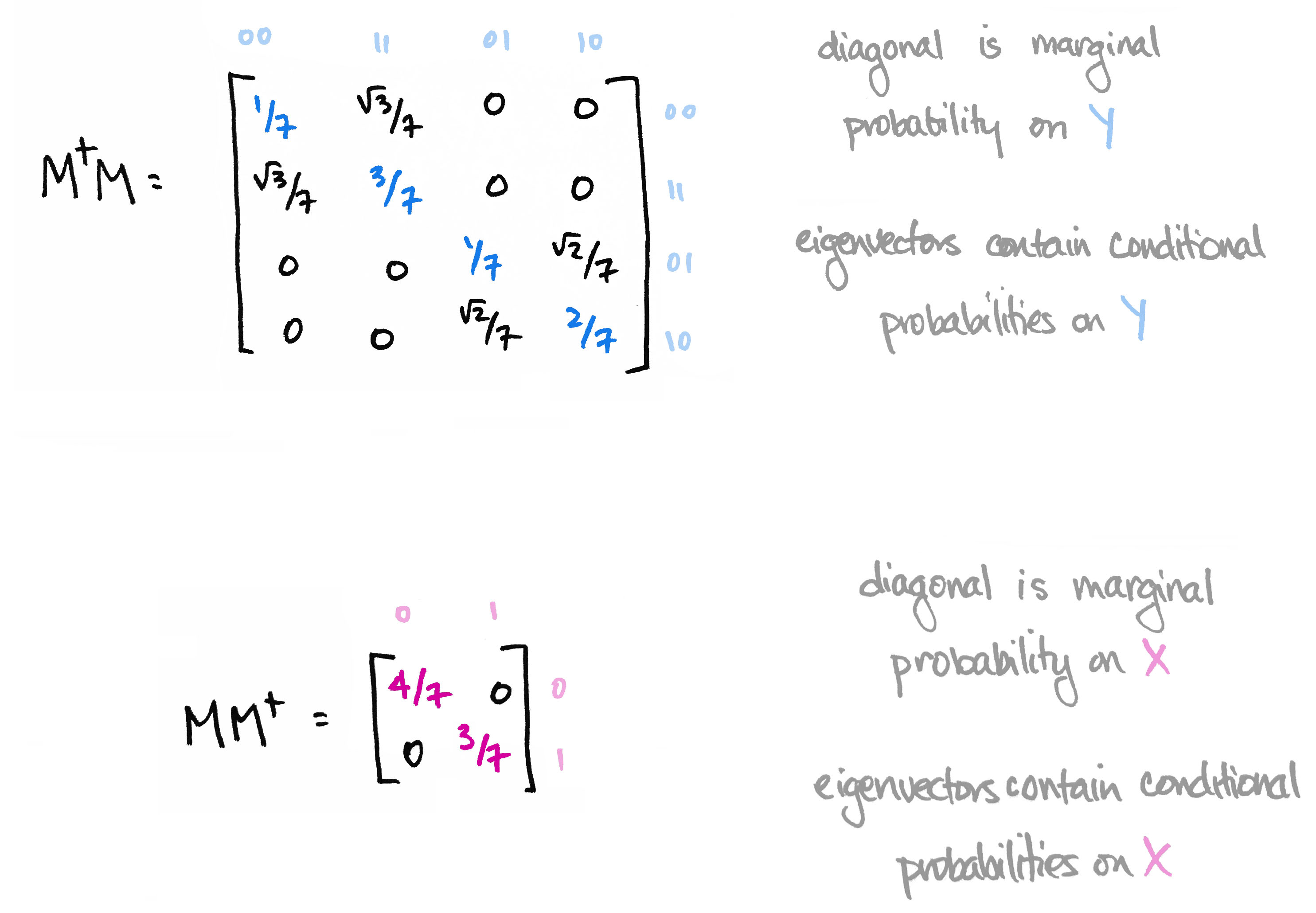
We then observed that the matrix $M^\top M$ contains the marginal probability distribution of $Y$ along its diagonal. Moreover its eigenvectors define conditional probability distributions on $Y$. Likewise, $MM^\top$ contains marginals on $X$ along its diagonal, and its eigenvectors define conditional probability distributions on $X$.

The information in the eigenvectors of $M^\top M$ and $MM^\top$ is precisely the information that's  destroyed when computing marginal probability in the usual way. The big reveal last time was that the matrices $M^\top M$ and $MM^\top$ are the quantum versions of marginal probability distributions.

As we'll see today, the quantum version of a probability distribution is something called a density operator. The quantum version of marginalizing corresponds to "reducing" that operator to a subsystem. This reduction is a construction in linear algebra called the partial trace. I'll start off by explaining the partial trace. Then I'll introduce the basics of quantum probability theory. At the end, we'll tie it all back to our bitstring example.

In this article and the next, I'd like to share some ideas from the world of quantum probability.* The word "quantum" is pretty loaded, but don't let that scare you. We'll take a first—not second or third—look at the subject, and the only prerequisites will be linear algebra and basic probability. In fact, I like to think of quantum probability as another name for "linear algebra + probability," so this mini-series will explore the mathematics, rather than the physics, of the subject.**

In today's post, we'll motivate the discussion by saying a few words about (classical) probability. In particular, let's spend a few moments thinking about the following: ‍

What do I mean? We'll start with some basic definitions. Then I'll share an example that illustrates this idea.

A probability distribution (or simply, distribution) on a finite set $X$ is a function $p \colon X\to [0,1]$ satisfying $\sum_x p(x) = 1$. I'll use the term joint probability distribution to refer to a distribution on a Cartesian product of finite sets, i.e. a function $p\colon X\times Y\to [0,1]$ satisfying $\sum_{(x,y)}p(x,y)=1$. Every joint distribution defines a marginal probability distribution on one of the sets by summing probabilities over the other set. For instance, the marginal distribution $p_X\colon X\to [0,1]$ on $X$ is defined by $p_X(x)=\sum_yp(x,y)$, in which the variable $y$ is summed, or "integrated," out. It's this very process of summing or integrating out that causes information to be lost. In other words, marginalizing loses information. It doesn't remember what was summed away!

I'll illustrate this with a simple example. To do so, I need to give you some finite sets $X$ and $Y$ and a probability distribution on them.

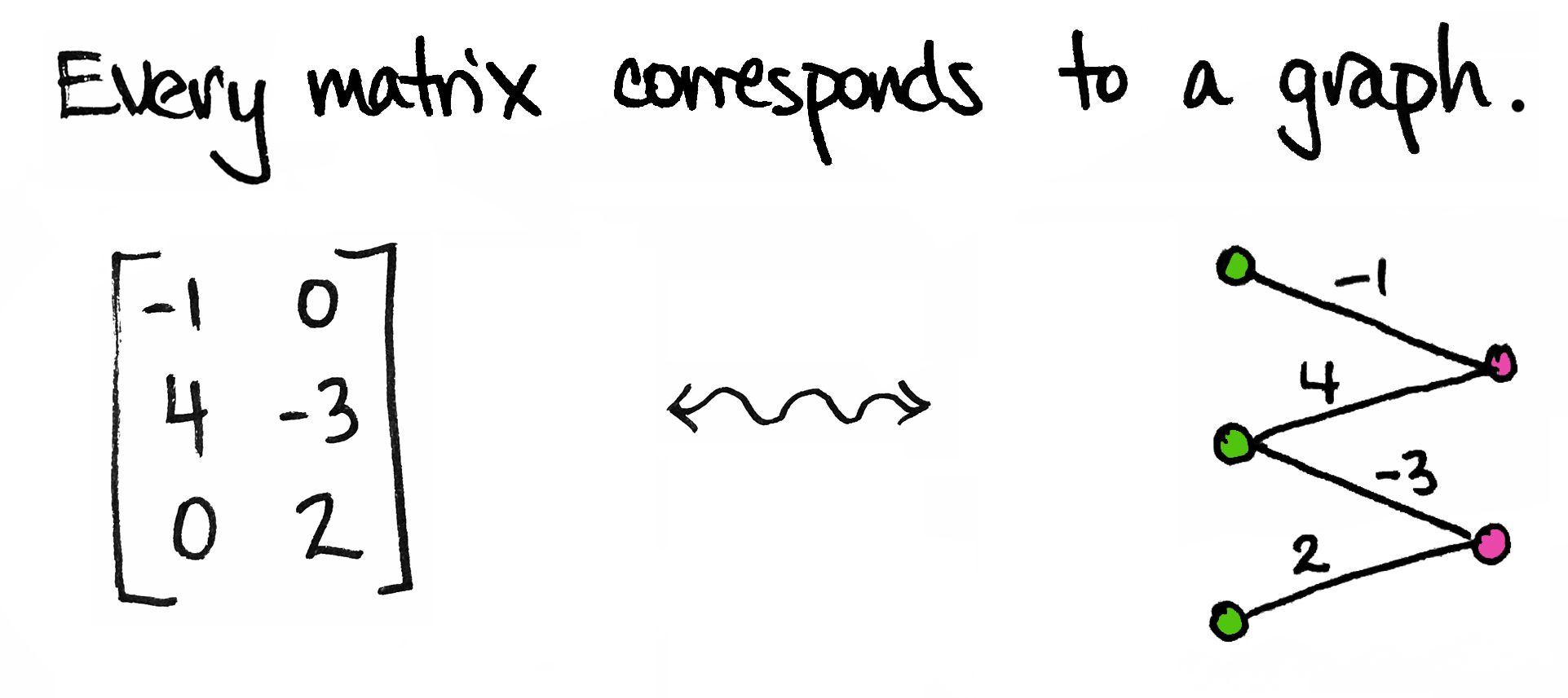
Today I'd like to share an idea. It's a very simple idea. It's not fancy and it's certainly not new. In fact, I'm sure many of you have thought about it already. But if you haven't—and even if you have!—I hope you'll take a few minutes to enjoy it with me. Here's the idea:

‍

So simple! But we can get a lot of mileage out of it.

To start, I'll be a little more precise: every matrix corresponds to a weighted bipartite graph. By "graph" I mean a collection of vertices (dots) and edges; by "bipartite" I mean that the dots come in two different types/colors; by "weighted" I mean each edge is labeled with a number.