In the past few months, I've shared a few mathematical ideas that I think are pretty neat: drawing matrices as bipartite graphs, picturing linear maps as tensor network diagrams, and understanding the linear algebraic (or "quantum") versions of probabilities.‍

These ideas are all related by a project I've been working on with Miles Stoudenmire—a research scientist at the Flatiron Institute—and John Terilla—a mathematician at CUNY and Tunnel. We recently posted a paper on the arXiv: "Modeling sequences with quantum states: a look under the hood," and today I'd like to tell you a little about it.

‍

Before jumping in, let's warm up with a question:

‍

Question: Suppose we have a set of data points drawn from a (possibly unknown) probability distribution $\pi$. Can we use the data points to define a new probability distribution that estimates $\pi$, with the goal of generating new data?

To illustrate this idea, here are a couple of examples.

Bitstrings

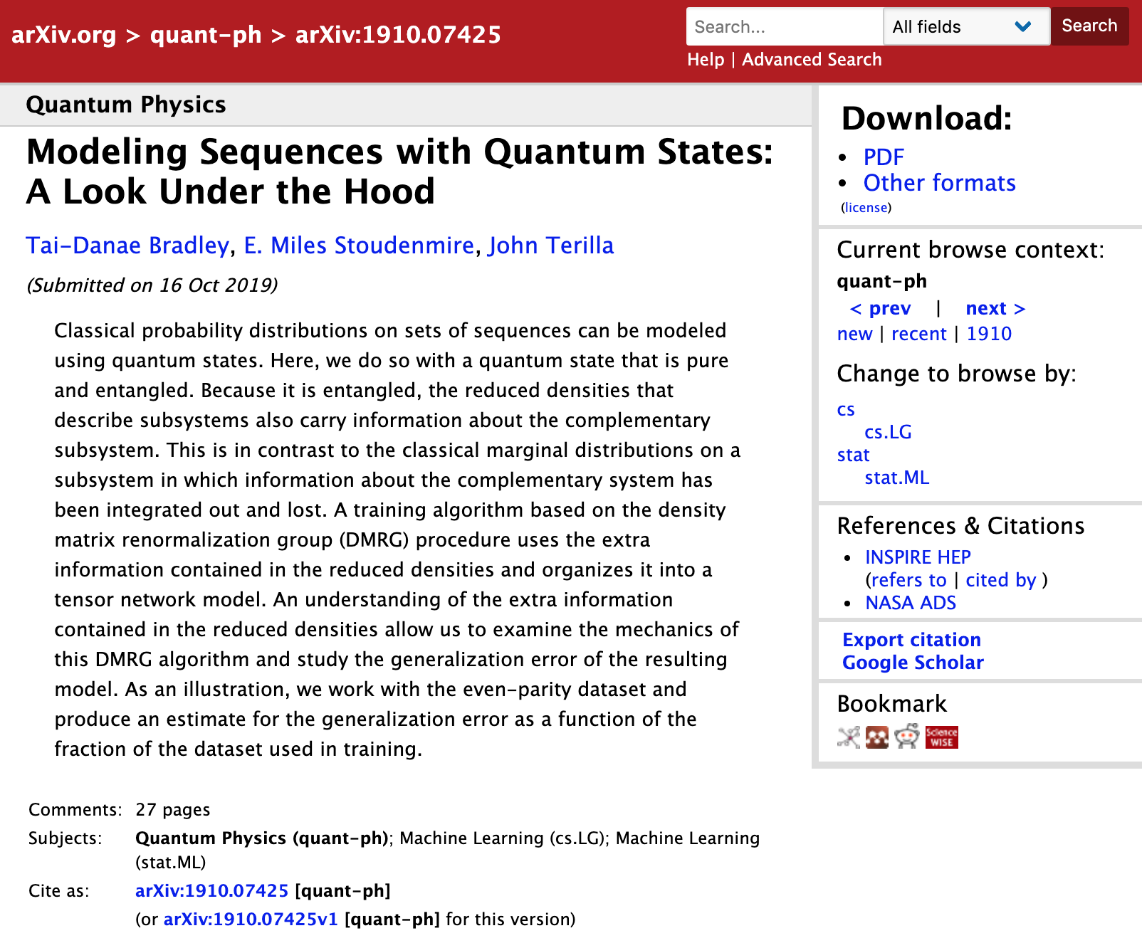
Suppose our data points are bitstrings—sequences of 0s and 1s—all of length $16$, for example. There are $2^{16}=65,536$ such strings, but suppose we only have a small fraction of them—a couple thousand, say—that we drew from some probability distribution $\pi$. We may or may not know what $\pi$ is, but either way we'd like to use information about the strings we do have in order to take a best guess at $\pi$. Once we have this best guess, we can generate new bitstrings by sampling from the distribution.

Natural language

Or suppose our data points are meaningful sentences—sequences of words from the English alphabet. There are tons of possibilities, but suppose we only have a small fraction of them—pages from Wikipedia or books from your local library. There is some probability distribution on natural language (e.g. the probability of "cute little dog" is higher than the probability of "tomato rickety blue"), though we don't have access to it. But we might like to use the data we do have to estimate the probability distribution on language in order to generate new, plausible text. That's what language models do.

These examples, I hope, help put today's blog post in context. We're interested in modeling probability distributions given samples from some dataset. There is mathematical theory that motivates the model, and there is a training algorithm to produce the model. What's more, it uses only basic tools from linear algebra, though I'll say more on that later.

Welcome to the last installment in our mini-series on adjunctions in category theory. We motivated the discussion in Part 1 and walked through formal definitions in Part 2. Today I'll share some examples. In Mac Lane's well-known words, "adjoint functors arise everywhere," so this post contains only a tiny subset of examples. Even so, I hope they'll help give you an eye for adjunctions and enhance your vision to spot them elsewhere.

An adjunction, you'll recall, consists of a pair of functors $F\dashv G$ between categories $\mathsf{C}$ and $\mathsf{D}$ together with a bijection of sets, as below, for all objects $X$ in $\mathsf{C}$ and $Y$ in $\mathsf{D}$.

In Part 2, we illustrated this bijection using a free-forgetful adjunction in linear algebra as our guide. So let's put "free-forgetful adjuctions" first on today's list of examples.

Last time I shared a light introduction to adjunctions in category theory. As we saw then, an adjunction consists of a pair of opposing functors $F$ and $G$ together with natural transformations $\text{id}\to\ GF$ and $FG\to\text{id}$. We compared this to two stricter scenarios: one where the composite functors equal the identities, and one where they are naturally isomorphic to the identities. The first scenario defines an isomorphism of categories. The second defines an equivalence of categories. An adjunction is third on the list.

In the case of an adjunction, we also ask that the natural transformations—called the unit and counit—somewhat behave as inverses of each other. This explains why the ${\color{red}\text{arrows}}$ point in opposite directions. (It also explains the "co.") Except, they can't literally be inverses since they're not composable: one involves morphisms in $\mathsf{C}$ and the other involves morphisms in $\mathsf{D}$. That is, their (co)domains don't match. But we can fix this by applying $F$ and $G$ so that (a modified version of) the unit and counit can indeed be composed. This brings us to the formal definition of an adjunction.

Some time ago, I started a "What is...?" series introducing the basics of category theory:

• "What is a category?"
• "What is a functor?" Part 1 and Part 2
• "What is a natural transformation?" Part 1 and Part 2

Today, we'll add adjunctions to the list. An adjunction is a pair of functors that interact in a particularly nice way. There's more to it, of course, so I'd like to share some motivation first. And rather than squeezing the motivation, the formal definition, and some examples into a single post, it will be good to take our time: Today, the motivation. Next time, the formal definition. Afterwards, I'll share examples.

Indeed, I will make the admittedly provocative claim that adjointness is a concept of fundamental logical and mathematical importance that is not captured elsewhere in mathematics.

- Steve Awodey (in Category Theory, Oxford Logic Guides)

Welcome back to our mini-series on quantum probability! Last time, we motivated the series by pondering over a thought from classical probability theory, namely that marginal probability doesn't have memory. That is, the process of summing over of a variable in a joint probability distribution causes information about that variable to be lost. But as we saw then, there is a quantum version of marginal probability that behaves much like "marginal probability with memory." It remembers what's destroyed when computing marginals in the usual way. In today's post, I'll unveil the details. Along the way, we'll take an introductory look at the mathematics of quantum probability theory.

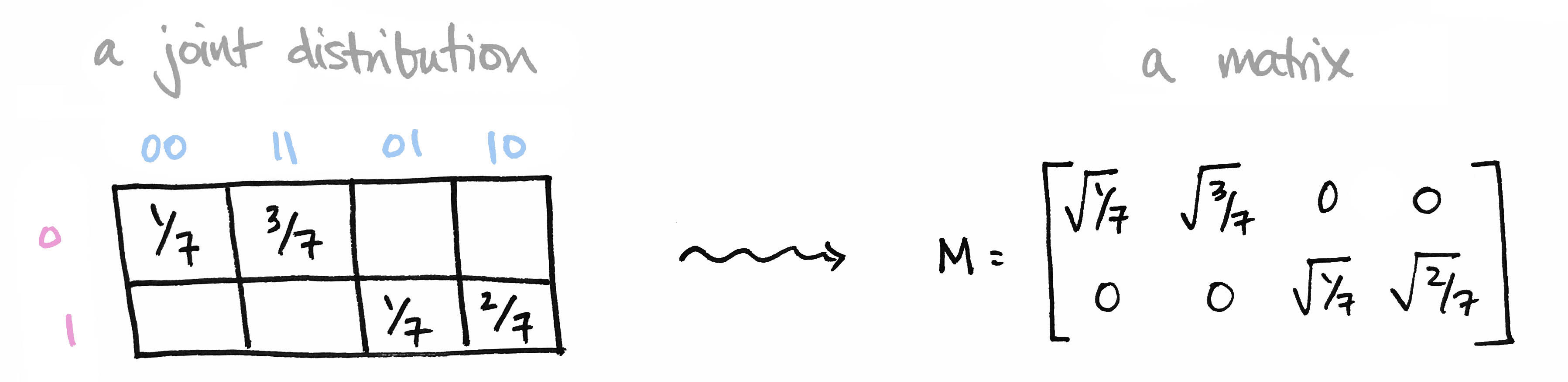
Let's begin with a brief recap of the ideas covered in Part 1: We began with a joint probability distribution on a product of finite sets $p\colon X\times Y\to [0,1]$ and realized it as a matrix $M$ by setting $M_{ij} = \sqrt{p(x_i),p(y_j)}$. We called elements of our set $X=\{0,1\}$ prefixes and the elements of our set $Y=\{00,11,01,10\}$ suffixes so that $X\times Y$ is the set of all bitstrings of length 3.

We then observed that the matrix $M^\top M$ contains the marginal probability distribution of $Y$ along its diagonal. Moreover its eigenvectors define conditional probability distributions on $Y$. Likewise, $MM^\top$ contains marginals on $X$ along its diagonal, and its eigenvectors define conditional probability distributions on $X$.

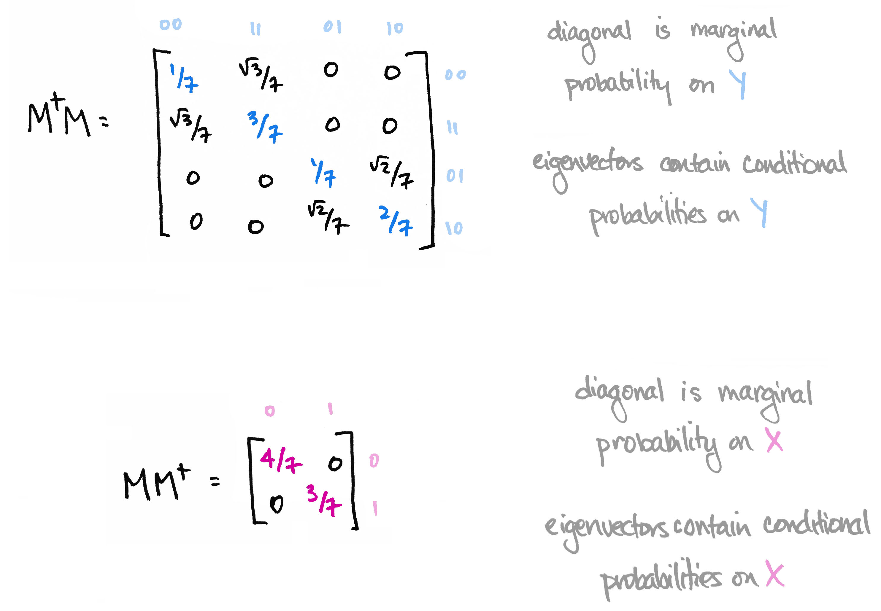
The information in the eigenvectors of $M^\top M$ and $MM^\top$ is precisely the information that's  destroyed when computing marginal probability in the usual way. The big reveal last time was that the matrices $M^\top M$ and $MM^\top$ are the quantum versions of marginal probability distributions.

As we'll see today, the quantum version of a probability distribution is something called a density operator. The quantum version of marginalizing corresponds to "reducing" that operator to a subsystem. This reduction is a construction in linear algebra called the partial trace. I'll start off by explaining the partial trace. Then I'll introduce the basics of quantum probability theory. At the end, we'll tie it all back to our bitstring example.